Implementing Character.AI’s Memory Optimizations in nanoGPT

20 Jan, 2025

Last year, the Character.AI team released a blog post that detailed their approach in building a highly efficient inference system that serves over 20,000 inference queries per second, roughly 20% of Google Search's traffic. They focused on reducing the KV Cache size, which plays a significant role in increasing the decoding speed in transformers, but is the key bottleneck in inference. Specifically, they implemented three model architecture changes which reduced the KV cache size by more than 20x. These techniques include Multi-Query Attention (MQA), Hybrid Attention Horizons, and Cross Layer KV-sharing.

In this blogpost, I am going to implement each of these memory optimizations into nanoGPT to measure both the theoretical and practical reductions in the KV cache size. I will be using GPT-2 small (124M) as my baseline model, and all training and inference will run on A100 GPUs via Lambda Labs. Below are the generation parameters and model architecture:

Baseline Model Architecture:
num_layers: 12 
num_heads: 12 
embedding_dim: 768 
dim_head: 64

Generation Parameters:
Number of Sequences: 10
Sequence Length: 1024
Precision: torch.float32

KV Cache Memory Usage in GPT-2 (124M)

The purpose of the KV Cache is to avoid recalculating the key and value vectors every time we sample a new token, and by caching the K and V vectors we can save a good amount of computation at the cost of some storage. The number of bytes we store in the KV Cache is:

KV Cache Size = 4 \times 2 \times n_{layers} \times n_{heads} \times {head}_{dim} \times sequence_length \times batch_size

4 represents the bytes in float32 precision, and 2 accounts for both the K and V vectors. Each layer in the model stores these vectors as $n_{heads} \times {head}_{dim}$ matrices. For inference, we set the $sequence_length$ to 1024 and our $batch_size$ to 1, and this gives us a theoretical KV Cache size of approximately 75.5MB. I previously implemented KV Cache in GPT2, and this will serve as our baseline model. To measure the total size, I’ll measure the peak memory usage during inference and compare runs with and without the KV Cache enabled.

Baseline Model:
Peak Memory Usage (MiB): 1279MiB

Baseline Model + KV Cache:
Peak Memory Usage (MiB): 1359MiB

The KV Cache is 80MB, which aligns with the theoretical size. Even in the smallest GPT-2 model, the KV cache is a significant memory cost, and this will grow significantly as we increase the model size, batch size and sequence length. For instance, GPT-3 with 175B parameters using the same sequence length of 1024 would require 4.5GB of memory for a single generation!

Multi-Query Attention (MQA)

Multi-Query Attention, designed by Character.AI founder Noam Shazeer, is an effective approach at reducing KV cache size. MQA modifies the attention blocks by allowing multiple query heads to share a single key/value head. This reduces the number of K/V heads significantly, which cuts down memory usage and maintains model accuracy.

In MQA, both the keys and values share a single head, and in our KV Cache size equation this simplifies to reducing $n_{heads}$ to 1. This drops our theoretical size down to 6.6MB!

description

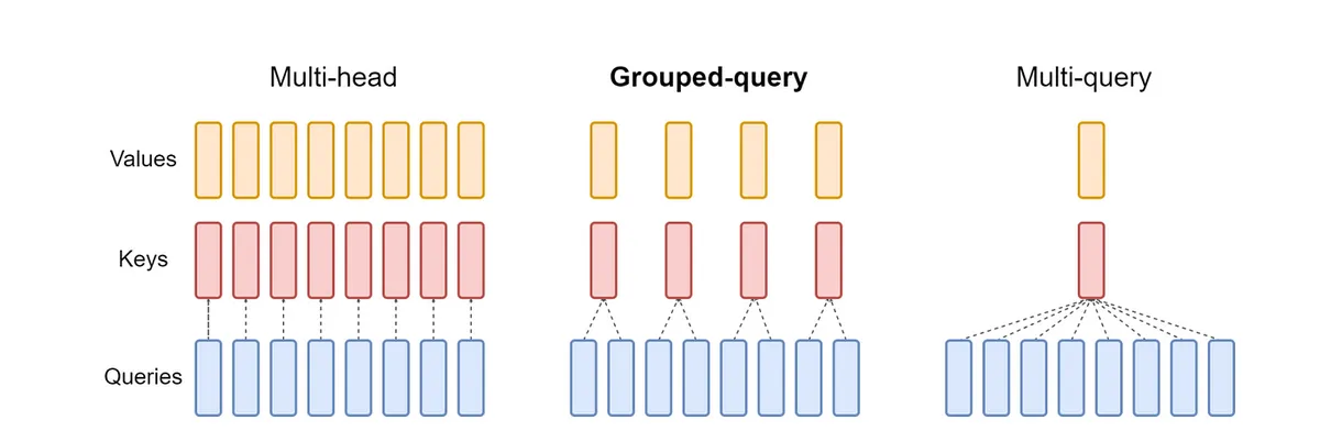
Source: GQA paper

To implement MQA into nanoGPT, we first add a new dimension n_kv_heads that represents the number of heads in key and value projections. For MQA, we set this to 1, but you could extend this for Grouped-Query Attention. Then in the attention class, we reduce our key and value projection layer sizes and keep the query projection unchanged. Finally, we reshape our Q, K, V tensors before calculating attention.

class CausalSelfAttention(nn.Module):
    def __init__(self, config, enable_local=False, enable_flash=False):
        
        # n_embd: embedding dimension (e.g. 768)
        # n_head: number of query heads (e.g. 12)
        # n_kv_heads: number of key/value heads (e.g. 1 for MQA, or 4 or 8 for GQA)

        ...
        
        # Calculate how many times each k/v head needs to be repeated 
        # MQA: n_head=12, n_kv_heads=1 -> n_rep=12 

        # Query heads: remains full size (all heads -> embed_dim)
        self.q_proj = nn.Linear(config.n_embd, config.n_embd)
        
        # Key/Value heads: Reduced size (fewer heads) 
        self.k_proj = nn.Linear(config.n_embd, (config.n_embd // config.n_head) * config.n_kv_heads)
        self.v_proj = nn.Linear(config.n_embd, (config.n_embd // config.n_head) * config.n_kv_heads)

        ...

    def forward(self, x, freqs_cos, freqs_sin, input_pos=None):
        B, T, C = x.size() # batch size, seq_length, embedding_dim
        # calculate query, key, values for all heads in batch
        q = self.q_proj(x)
        k = self.k_proj(x) 
        v = self.v_proj(x)

        # Reshape tensors for attention calculation [B, T, C]  (batch, seq_length, embedding_dim)
        q = q.view(B, T, self.n_head, C // self.n_head).transpose(1, 2) # (B, nh, T, hs)
        k = k.view(B, T, self.n_kv_heads, C // self.n_head).transpose(1, 2) # (B, nkvh, T, hs)
        v = v.view(B, T, self.n_kv_heads, C // self.n_head).transpose(1, 2) # (B, nkvh, T, hs)
        
        ...

The K/V tensors end up with fewer heads than the query tensor after reshaping. To match the shapes, we define a repeat_kv() function that broadcasts the K/V tensors n_head/n_kv_head times, and for MQA we repeat this 12 times. The broadcasting operation creates a view of the original tensor without allocating new memory for the repeats.

Note that the KV Cache operation happens before we broadcast the key and value heads. In our model, we only cache tensors with a single K/V head, which significantly reduces the memory usage. After the cache operation, we broadcast this compressed tensor to match the number of query heads for the attention calculation.

def repeat_kv(x: torch.Tensor, n_rep: int) -> torch.Tensor:
    # Expands each K/V head to match the number of query heads 
    # MQA: n_kv_heads=1, n_head=12 -> K/V head is repeated 12 times
    
    bs, n_kv_heads, slen, head_dim = x.shape
    
    # Shape Gymnastics 🤸‍♀️
    return (
        x[:, :, None, :, :]
        .expand(bs, n_kv_heads, n_rep, slen, head_dim)  # [bs, n_kv_heads, n_rep, slen, head_dim]
        .reshape(bs, n_kv_heads * n_rep, slen, head_dim) 
    )

class CausalSelfAttention(nn.Module):
... 

    def forward(self, x, freqs_cos, freqs_sin, input_pos=None):
        ...

        # Store/retrieve compressed K/V tensors for KV cache 
        if self.kv_cache is not None and input_pos is not None:
            k, v = self.kv_cache.update(input_pos, k, v)

        # After KV Cache operation, expand K/V tensors to match query heads 
        k = repeat_kv(k, self.n_rep)
        v = repeat_kv(v, self.n_rep)
        
        # Compute attention 
        y = q * k.transpose(-2, -1) # attention scores
        
        # Final projection
        y = y.transpose(1, 2).contiguous().view(B, T, C)
        y = self.c_proj(y)

RoPE detour

Before moving on, I thought it would be a disservice to the "NOAM" architecture if I skipped RoPE. I won't go too deep into details since there are many great resources online. The key thing to know is that RoPE encodes the relative position dynamically. Absolute positional embeddings directly add position values to the token embeddings, which creates two problems. First, the absolute positions matters far less than the relative position, we care more about how words relate to their neighbors than if this word is the 107th in a paragraph. Second, by directly adding the absolute position information to the token embeddings, we risk diluting the semantic information of a token.

Instead of adding information directly to the token’s magnitude, RoPE directly encodes relative positions into the attention calculation. RoPE rotates the key and query vectors during attention via a rotation matrix, and this approach preserves the token's semantic information while encoding the distance between tokens.

description

Source: Chris Fleetwood

You can still implement MQA with GPT2's learned positional embeddings, but RoPE is better for memory optimization. RoPE calculates positions using $s i n$ and $c o s$ functions on the fly, which eliminates the need for a dedicated embedding table. While removing the positional embedding table saves a relatively small number of parameters, at Character.AI’s query volume, this minor optimization is significant. Moreover, the memory-optimizations in this model architecture fit well with RoPE. We don't need to store and compress a position table, and we can still encode the relative position accurately in the attention layers.

To implement RoPE, there are two key functions. The first function is precomputing the position-based rotation values via precompute_freqs_cis(). We first create the frequency bands for each embedding dimension pair, and these control how quickly each pair rotates via the $w_{i} = \frac{1}{10000^{2 i / d}}$ , where $θ = 10000$ controls the base rotation rate. Then, we multiply each position by these frequencies, so position $p$ gets multiplied by each $ω ᵢ$ to get $p ω ᵢ$ . We can then calculate the $c o s$ and $s i n$ of these angles to get the rotation matrix for each position-dimension pair.

𝐌_{i} = [\begin{matrix} \cos (ω_{i} p) & \sin (ω_{i} p) \\ - \sin (ω_{i} p) & \cos (ω_{i} p) \end{matrix}]

def precompute_freqs_cis(dim: int, end: int, theta: float = 10000.0):
    # Calculate frequency bands for each dimension pair ->  ωᵢ = 1/theta^(2i/d)
    freqs = 1.0 / (theta ** (torch.arange(0, dim, 2)[: (dim // 2)].float() / dim))
    t = torch.arange(end, dtype=torch.float)
    
    # Multiply position indices by frequencies
    freqs = torch.outer(t, freqs)  
    
    # Create rotary position embedding components 
    cos = torch.cos(freqs) 
    sin = torch.sin(freqs)
    
    return cos, sin

class GPTMQA(nn.Module):
    def __init__(self, config):
        ...
        
        # Get rotary embedding angles for each position/dimension -> [cos(pθ), sin(pθ)]
        self.freqs_cos, self.freqs_sin = precompute_freqs_cis(
            config.n_embd // config.n_head,
            config.block_size,
            config.rope_theta,
        )

The second function applies our rotation matrix to the query and key projections via RoPE. We split our q and k vectors into pairs and encode relative positions by multiplying each dimension pair with the rotation matrix.

R (𝐪, p) = (\begin{matrix} 𝐌_{1} \\ 𝐌_{2} \\ ⋱ \\ 𝐌_{d / 2} \end{matrix}) (\begin{matrix} q_{1} \\ q_{2} \\ ⋮ \\ q_{d} \end{matrix})

For more efficient computation, we can avoid the sparse rotation matrix calculation, and instead directly apply the precomputed rotation pairs to each dimension pair in our queries and keys independently.

R_{Θ, p}^{d} q = (\begin{matrix} q_{1} \\ q_{2} \\ q_{3} \\ q_{4} \\ ⋮ \\ q_{d - 1} \\ q_{d} \end{matrix}) \otimes (\begin{matrix} \cos p θ_{1} \\ \cos p θ_{1} \\ \cos p θ_{2} \\ \cos p θ_{2} \\ ⋮ \\ \cos p θ_{d / 2} \\ \cos p θ_{d / 2} \end{matrix}) + (\begin{matrix} - q_{2} \\ q_{1} \\ - q_{4} \\ q_{3} \\ ⋮ \\ - q_{d} \\ q_{d - 1} \end{matrix}) \otimes (\begin{matrix} \sin p θ_{1} \\ \sin p θ_{1} \\ \sin p θ_{2} \\ \sin p θ_{2} \\ ⋮ \\ \sin p θ_{d / 2} \\ \sin p θ_{d / 2} \end{matrix})

First we split the input query/key tensors into two components and then reshape the frequency tensors to match the Q/K dimensions. We then independently apply the $c o s$ and $s i n$ rotations to each of the 2D pairs in our query and key vectors, which is more efficient. Next, we call apply_rotary_emb() in our attention equation on the query and key vectors, which now embeds the relative position directly into our attention formula. Finally, we remove the learned positional embedding table from nanoGPT.

Note that we apply rotary embeddings before repeating the key and value tensors. This makes sure that we apply the positional encodings to our compressed K/V representations first. These position-encoded K/V tensors then go into the KV Cache, which are then broadcast to match the query heads in the attention formula.

def apply_rotary_emb(x, freqs_cos, freqs_sin):
    
    # x shape: (bs, n_heads, seqlen, head_dim) -> (4, 32, 8, 128)
    # freqs_cos shape: (seq_len, head_dim//2) -> (8, 64)
    # freqs_sin shape: (seq_len, head_dim//2) -> (8, 64)
    
    # Separate the even and odd dimensions in x
    x1 = x[..., ::2]  # (bs, n_heads, seqlen, head_dim//2)
    x2 = x[..., 1::2]  # (bs, n_heads, seqlen, head_dim//2)
    
    # Reshape freqs_cos and freqs_sin to match x's dimension
    seq_len, rotation_dim = freqs_cos.shape
    freqs_cos = freqs_cos.view(1, 1, x.size(2), -1)  # (1, 1, seqlen, rotation_dim)
    freqs_sin = freqs_sin.view(1, 1, x.size(2), -1)  # (1, 1, seqlen, rotation_dim)

    # Apply rotary embeddings
    x_out1 = x1 * freqs_cos - x2 * freqs_sin  # Rotate first half
    x_out2 = x2 * freqs_cos + x1 * freqs_sin  # Rotate second half

    # Combine rotated halves back together
    return torch.stack((x_out1, x_out2), dim=-1).flatten(-2)

class CausalSelfAttention(nn.Module):
    ...
    def forward(self, x, freqs_cos, freqs_sin, input_pos=None):
        
        ...
        
        # Apply rotary embeddings to query and key vectors
        q = apply_rotary_emb(q, freqs_cos, freqs_sin)
        k = apply_rotary_emb(k, freqs_cos, freqs_sin)

        # Then update the KV Cache
        if self.kv_cache is not None and input_pos is not None:
            k, v = self.kv_cache.update(input_pos, k, v)

        # Then broadcast to match the query heads
        k = repeat_kv(k, self.n_rep)
        v = repeat_kv(v, self.n_rep)

        ...

Hybrid Attention Horizons (Sliding Window)

The second memory optimization Character.AI involves interleaving "local" attention layers with global attention layers, where every 6th layer in the model is a global attention layer. Global attention is just normal causal attention where each token can attend to every other token in the sequence, which leads to $O (n^{2})$ complexity. Local attention restricts each token to attend to a fixed sliding window length (1024 in Character.AI). This window slides along with the position in the sequence, and tokens can only attend to others within the current window. This sliding window approach reduces complexity to $O (n)$ . This method was popularized in the Mistral 7B paper, where the authors argue that recent tokens are more valuable for predicting the next word in a sequence.

description

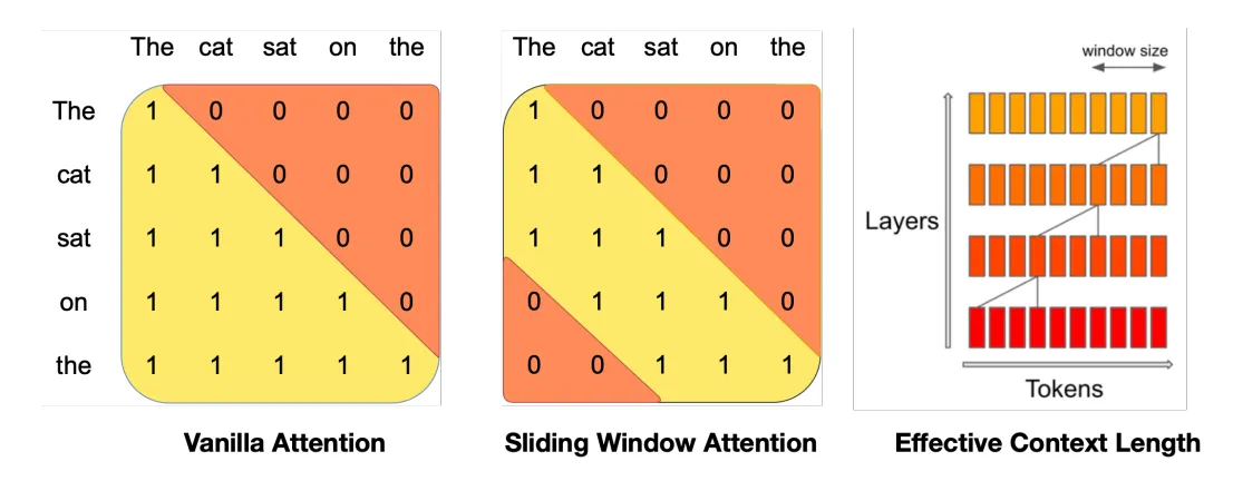
Source: Mistral 7B paper

To implement local attention we combine two different masks, which are the causal and sliding window mask. The causal mask (vanilla attention) prevents tokens from attending to future positions, and the sliding window mask restricts each token to only attend to nearby tokens within its window. By taking the intersection of these masks, we create a local attention mask that ensures each token can only attend to itself and the fixed window of past tokens.

Causal Mask:
1 . . . . . . .    
1 1 . . . . . .    
1 1 1 . . . . .    
1 1 1 1 . . . .    
1 1 1 1 1 . . .    
1 1 1 1 1 1 . .    
1 1 1 1 1 1 1 .    
1 1 1 1 1 1 1 1    

Sliding Window Mask:
1 1 1 . . . . .    
1 1 1 1 . . . .    
. 1 1 1 1 . . .    
. . 1 1 1 1 . .    
. . . 1 1 1 1 .    
. . . . 1 1 1 1    
. . . . . 1 1 1    
. . . . . . 1 1    

Sliding Window Mask + Causal Mask:
1 . . . . . . .    
1 1 . . . . . .    
. 1 1 . . . . .    
. . 1 1 . . . .    
. . . 1 1 . . .    
. . . . 1 1 . .    
. . . . . 1 1 .    
. . . . . . 1 1

Unfortunately, combining these masks creates a sparse attention pattern, which leads to irregular memory access patterns that are cache unfriendly. GPUs perform best with dense, continuous memory patterns that allow for efficient memory access, and the sliding window attention mask has scattered attention positions that result in poor memory access. This sparsity exists in the standard causal attention also, and Flash Attention addresses this through fused CUDA kernels that efficiently handle the causal mask without materializing the full sparse matrix in GPU memory. However, FlashAttention isn’t flexible for other attention variants, and we would need to write a custom kernel on top of FlashAttention to get SWA working.

FlexAttention solves this issue by providing an API to define custom attention masks while still maintaining high performance. We convert our custom attention mask through torch.compile into optimized CUDA kernels automatically. FlexAttention then translates the mask into Triton code and injects it directly into FlashAttention kernel templates for both the forward and backward passes. This approach gives us about 90% of FlashAttention2's forward pass performance and 85% of its backward pass performance, and we don't have to write any kernels! We can now implement sliding window attention efficiently while any manual kernel optimizations.

To implement sliding window attention, we use FlexAttention's mask_mod and create_block_mask() function to generate a mask for our attention calculation. The mask_mod optimizes computation by skipping masked-out values in our sparse attention matrix, and only computing attention within our fixed window. I chose a WINDOW_SIZE of 256 for our 1024 context length, and this factor of 4 stems from Mistral 7B, where they used a 4096 window for a 16K context length.

WINDOW_SIZE = 256
def sliding_window_causal(self, b, h, q_idx, kv_idx):
    causal_mask = q_idx >= kv_idx
    window_mask = q_idx - kv_idx <= WINDOW_SIZE
    return causal_mask & window_mask

class CausalSelfAttention(nn.Module):
...
    def forward(self, x, freqs_cis, input_pos=None):
        ...
        
        # Create block mask for sliding window
        if self.local_attention:
            block_mask = create_block_mask(
                sliding_window_causal,
                B,                          # Batch size
                self.n_head,                # Number of heads
                T,                          # Query sequence length
                T,                          # Key/value sequence length
                device=x.device
            )
            y = flex_attention(q, k, v, block_mask=block_mask)
        else:
            # normal causal attention - use Flash Attention here
            ... 
        
        # final projection
        y = y.transpose(1, 2).contiguous().view(B, T, C)
        y = self.c_proj(y)
        return y

We now intersperse global and local attention layers into our model architecture. For every 6th layer, we insert a global attention layer that uses FlashAttention, and every other layer uses local attention with SWA. We set this up by passing in an enable_local bool every 5 layers and use the converse of that to set FlashAttention.

class Block(nn.Module):
    def __init__(self, config, use_local=True):
        super().__init__()
        self.ln_1 = nn.LayerNorm(config.n_embd)
        self.attn = CausalSelfAttention(config, enable_local=use_local, enable_flash=not use_local)
        self.ln_2 = nn.LayerNorm(config.n_embd)
        self.mlp = MLP(config)

    ...

class GPTMQA(nn.Module):
    def __init__(self, config):
        ...
        self.transformer = nn.ModuleDict(dict(
            wte = nn.Embedding(config.vocab_size, config.n_embd),
            h = nn.ModuleList([
                Block(config, use_local=(i % 6 != 0)) for i in range(config.n_layer)
            ]),
            ln_f = nn.LayerNorm(config.n_embd, eps=config.norm_eps),
        ))
        self.lm_head = nn.Linear(config.n_embd, config.vocab_size, bias=False)
        self.transformer.wte.weight = self.lm_head.weight # weight tying

The final change the Character.AI team makes is cross layer KV-sharing, where they tie K and V heads between neighboring attention layers, which reduces the KV Cache size further by 2-3x.

description

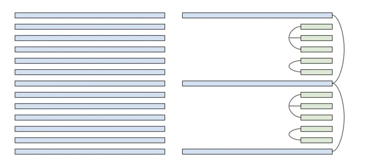
Source: Character.AI

There are two approaches in terms of tying K and V layers. The first one is sharing the K and V heads across layers during training using Cross Layer Attention. This benefits in aligning your forward pass between training and inference, which reduces any inference mismatches. To implement this approach, you would need to persist previous k and v states at each layer, and then control the number of shared layers that contain the same projections.

class CrossLayerAttention(nn.Module):
    def __init__(self, config, shared_layers):
        ...
        self.shared_layers = shared_layers
        self.attn = CausalSelfAttention(config)
        
        # Create shared key/value projections
        self.kv_proj = nn.Linear(config.n_embed, config.n_embed * 2)
        self.q_proj = nn.Linear(config.n_embed, config.n_embed)

    def forward(self, x, prev_kv=None):
        # if previous k_v layers stored, reuse for attention computation
        if prev_kv is None:
            kv = self.kv_proj(x)
            k, v = torch.chunk(kv, 2, dim=-1)
        else:
            k, v = prev_kv
                
        # calculate normal attention 
        # you would need to modify CausalSelfAttention 
        # to pass in precomputed k and v values
        attn = self.attn(x, pre_k=k, prev_v=v)


class Block(nn.Module):
    def __init__(self, config, shared_layers=2):
        # local attention -> 2,3 shared_layers
        # global attention -> 2 shared_layers
        self.attn = CrossLayerAttention(config, shared_layers)
        
        ...
        self.shared_layers = shared_layers
        self.prev_kv = None

    def forward(self, x):
        # reuse previous k and v layers to compute attention
        if self.prev_kv is None or self.shared_layers <= 1:
            x, self.prev_kv = self.attn(x)
        else:
            x = self.attn(x, prev_kv=self.prev_kv)

The second approach, which I chose for my implementation, just ties the KV Cache during inference. In the model, local caches are shared together and global caches are tied separately. Global attention layers take up most of the KV Cache size in long context inference, so tying these caches shows improved memory performance.

In my experiments, I found that there were minimal quality differences between the two approaches, and slightly better memory reduction in tying KV caches. There has been some similar work done in recent papers, and my initial thought is because nanoGPT only has 12 layers, there wouldn’t be too many alignment differences between training and inference anyway. However, if you are training larger models, it is probably better to do the first approach.

I structured my implementation into two phases. First I set up individual KV Caches for each layer in my model, and then I tied the caches together. I thought this was easier to follow than trying to tie them in one step, and it also enables ablation studies to test the impact. As shown above, I followed Character.AI’s specific grouping pattern, which was tying the first two local attention layers, the next three local attention layers¹, and then the global attention layers. This pattern was then repeated for all 12 layers in our model.

Below are my implementations for setting up the caches at each layer and tying them afterwards. I also included a verification function to check if the layers are sharing the same memory address for a KV cache object.

def setup_caches(self, max_batch_size, max_seq_length):
    ...
    
    # Create new KV (Key-Value) cache for each transformer attention layer
    for block in self.transformer.h:
        block.attn.kv_cache = KVCache(
            max_batch_size=max_batch_size,        # Max # of sequences to process at once
            max_seq_length=max_seq_length,        # Max length of each sequence
            n_kv_heads=self.config.n_kv_heads,    # Use n_kv_heads instead of n_head
            head_dim=head_dim,                    # head dimension
            dtype=dtype                           # Current dtype comes from the output layer
        )


def tie_kv_caches(self):

    # Global layer occurs every 6th layer
    global_layers = [i for i in range(len(self.transformer.h)) if i % 6 == 0]
    
    # Tie global layer caches
    if global_layers:
        shared_global_cache = self.transformer.h[global_layers[0]].attn.kv_cache
        for layer_idx in global_layers[1:]:
            self.transformer.h[layer_idx].attn.kv_cache = shared_global_cache
    
    # Get local layers    
    local_groups = [list(range(i+1, min(i+6, len(self.transformer.h)))) for i in global_layers]
    
    for group in local_groups:
        # First three layers share cache
        if len(group) >= 3:
            shared_cache = self.transformer.h[group[0]].attn.kv_cache
            self.transformer.h[group[1]].attn.kv_cache = shared_cache
            self.transformer.h[group[2]].attn.kv_cache = shared_cache
        
        # Last two local layers share cache
        if len(group) >= 5:
            shared_cache = self.transformer.h[group[3]].attn.kv_cache
            self.transformer.h[group[4]].attn.kv_cache = shared_cache


def verify_kv_sharing():
    
    # Verify Global Layer Sharing        
    global_layers = [i for i in range(len(self.transformer.h)) if i % 6 == 0]
    base_cache = get_cache_id(global_layers[0])
    for layer in global_layers:
        verify_same_cache(layer.cache_id, base_cache)
    
    # Verify Local Layer Groups
    for block_start in global_layers:
        layers_1_to_3 = [block_start + 1, block_start + 2, block_start + 3]
        base_cache = get_cache_id(layers_1_to_3[0])
        verify_same_cache(layers_1_to_3, base_cache)
    
        layers_4_to_5 = [block_start + 4, block_start + 5]
        base_cache = get_cache_id(layers_4_to_5[0])
        verify_same_cache(layers_4_to_5, base_cache)

Final Model Performance

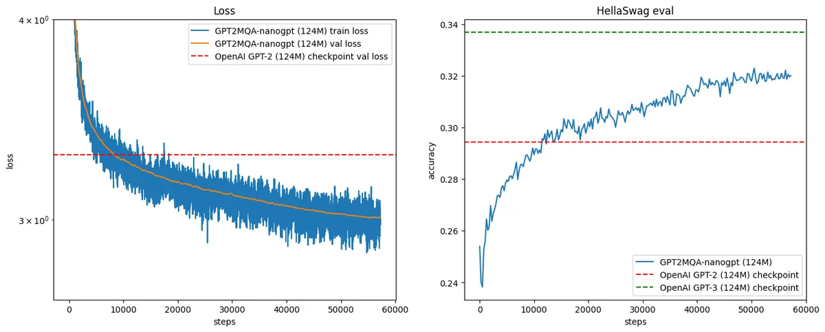
I used the same training recipe from Karpathy's GPT-2 reproduction video, which was training on the FineWeb-Edu dataset and evaluating with the Hellaswag benchmark. After training on 30B tokens, our modified GPT-2 model achieved similar validation loss and Hellaswag scores to the original nanoGPT model.

description

I then used the same generation parameters from the beginning to measure the size of the KV Cache with Cross Layer KV-sharing.

Final Model:
Peak Memory Usage (MiB): 1190MiB

Final Model + KV Cache:
Peak Memory Usage (MiB): 1196MiB

Final Model + KV Cache + Cross Layer KV-sharing:
Peak Memory Usage (MiB): 1192MiB

Our final model achieves a KV Cache size of 2MB, a 40x reduction to the baseline model! Moreover, enabling Cross Layer KV-sharing further reduces our cache size by 3x. If we scaled this model to GPT-3’s size with 175B parameters, the KV Cache for an inference call now would only require 115.2MB.

Conclusion

In the future, there are several other memory optimizations and inference speed techniques the Character.AI team implements that I think are worth exploring.

Stateful Caching: They developed an inter-turn cache system that stores KV values in a LRU Cache, similar to RadixAttention. This is a system-level improvement between chat turns, and it could be worth exploring if we implement our nanoGPT model in a chat-based system.
Native int8 training + kernels speedups: Character.AI doesn't reveal much about their int8 quantization techniques unfortunately. They train models natively in int8 precision and use custom int8 kernels for faster inference, which is detailed in their second blogpost. Though libraries like Google's AQT and torchao offer some int8 training approaches, we would need to wait for a more detailed report to understand their complete methodology.

Special thanks to the FlexAttention authors for their Sliding Window implementation, Andrej Karpathy for his nanoGPT repo, and the Character.AI team for their initial report that inspired this article.

My naive hypothesis is that we could optimize this further using powers of 2, which typically align better with memory operations. Instead of having three layers share a single KV Cache, adding an extra local attention layer might improve performance.↩

Implementing Character.AI’s Memory Optimizations in nanoGPT

KV Cache Memory Usage in GPT-2 (124M)

Multi-Query Attention (MQA)

RoPE detour

Hybrid Attention Horizons (Sliding Window)

Cross Layer KV-Sharing

Final Model Performance

Conclusion